m_fe <- feols(dpd30 ~ raised | SK_ID_PREV, data = d, cluster = ~SK_ID_PREV)5 Comparing an account with itself
What a fixed effect is underneath
Chapter 4 failed because the thing separating the two groups was never measured. So stop comparing groups.
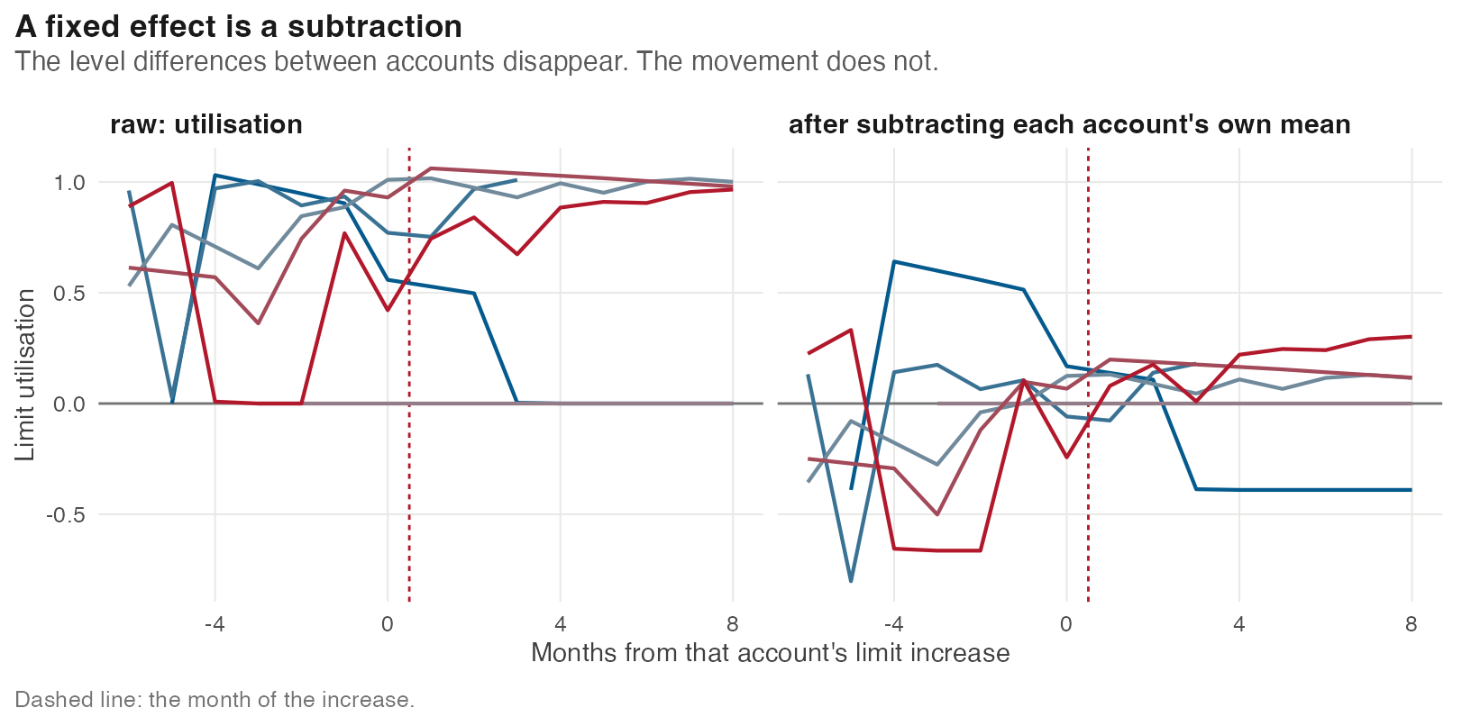
Every treated account appears in the data both before and after its own increase. Compare those two stretches and whatever is constant about that customer — their discipline, their job stability, the assessment the lender made — is identical on both sides. It cancels. We never have to know what it was.
5.1 The estimate
                      Model Estimate (pp) SE (pp)      t
                     <char>        <char>  <char> <char>
1: Pooled OLS + utilization        -1.272   0.045  -28.3
2:     Account fixed effect        +0.019   0.015    1.3
The sign flips. Not because the data changed — because the comparison did.
5.2 Why subtracting a mean removes the customer
Write down what we think is happening. For account \(i\) in month \(t\):
\[ y_{it} \;=\; \beta\, x_{it} \;+\; \alpha_i \;+\; \varepsilon_{it} \]
\(y\) is delinquency, \(x\) is whether the limit has been raised, and \(\beta\) is what we want. \(\alpha_i\) is everything about that customer that does not change: their discipline, their job stability, the assessment the lender made when it decided to trust them. We cannot measure it. It is one number per account, the same in every month.
Now average that whole equation over the months of account \(i\):
\[ \bar{y}_i \;=\; \beta\, \bar{x}_i \;+\; \alpha_i \;+\; \bar{\varepsilon}_i \]
\(\alpha_i\) comes through untouched. Averaging a number that never changes gives back the same number — that is the only property of \(\alpha_i\) we use, and it is why “time-invariant” is the whole requirement.
Subtract the second line from the first:
\[ y_{it} - \bar{y}_i \;=\; \beta\,(x_{it} - \bar{x}_i) \;+\; \underbrace{(\alpha_i - \alpha_i)}_{=\,0} \;+\; (\varepsilon_{it} - \bar{\varepsilon}_i) \]
The unmeasured customer is gone, and \(\beta\) is untouched. That is the entire trick.
The subtraction applies to every variable, not just the treatment
This is the part that trips people up. We are not doing something special to raised. We subtracted the same quantity — account \(i\)’s own average — from both sides of one equation, so every variable in it gets the same treatment: the outcome, the regressor, and any controls you had added.
In the code below that is two lines because this regression has two variables. Add a control and it would be three. What makes \(\alpha_i\) disappear is not which variable you demean, it is that you demeaned the whole equation.
In plain words, the regression now asks each account a question about itself: in your months on a raised limit, were you more often in arrears than in your own typical month? It never asks how you compare with anybody else.
5.3 It is a subtraction, not a black box
| SK_ID_PREV looks like an instruction to a solver. It is arithmetic. Subtract each account’s own average from every variable, then run ordinary least squares on the remainder:
d[, y_dm := dpd30  - mean(dpd30),  by = SK_ID_PREV]
d[, x_dm := raised - mean(raised), by = SK_ID_PREV]
by_hand <- lm(y_dm ~ x_dm - 1, data = d) Method Estimate (pp)
<char> <char>
1: demeaned by hand, then lm() 0.018556
2: feols(dpd30 ~ raised | SK_ID_PREV) 0.018556They agree to 4e-14 pp, which is floating-point noise.
The account effect is constant over time, so it equals its own average, so it disappears when you subtract that average. That is the entire trick — and it is why the unmeasured judgement from chapter 2 stops mattering. You do not need to observe something in order to subtract it, as long as it does not move.
But not every account can answer that question. Which ones do?
Where this chapter’s code lives
Everything above runs from 05-subtracting.qmd. Shared setup R/_common.R. The panel itself is built by R/01-build.R.