ks <- setdiff(-6:8, -1)                     # month -1 is the baseline
for (kk in ks) d[, paste0("m", kk + 9) := as.integer(!is.na(k) & k == kk)]
terms_ <- paste0("m", ks + 9)

by_month <- feols(
  as.formula(paste("dpd30 ~", paste(terms_, collapse = " + "),
                   "| SK_ID_PREV + MONTHS_BALANCE")),
  data = d, cluster = ~SK_ID_PREV)

prof <- data.table(k = ks, est = 100 * coef(by_month)[terms_], se = 100 * se(by_month)[terms_])
prof <- rbind(prof, data.table(k = -1L, est = 0, se = 0))[order(k)]9 Why believe it
Two checks: does it behave like a real effect?
The number is small and it came out of a long chain of subtractions. Two checks are worth running before trusting it, and both ask the same thing: does it behave the way a real effect would behave?
9.1 It appears only after the increase
If this were selection dressed up as an effect — accounts already drifting into trouble, and the lender happening to raise their limits — the drift would be visible before the event too. So estimate a separate coefficient for each month around the increase instead of one average.
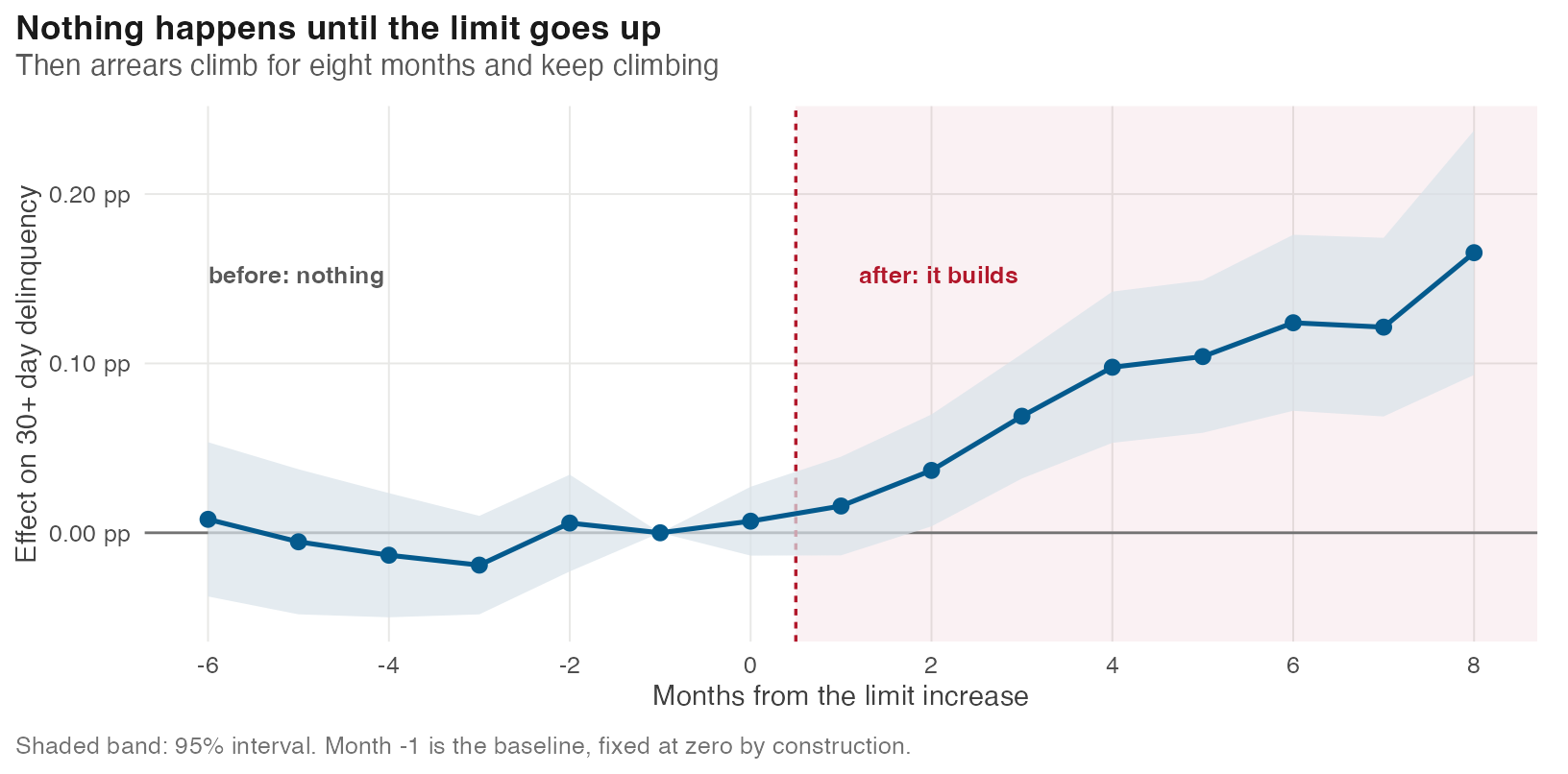
Every coefficient before the event sits within ±0.019 pp of zero and none is significant. After it, the effect grows month by month to +0.165 pp.
That shape is hard to fake. Selection produces a gap that is already there; it does not wait for the event and then ramp up over eight months.
9.2 A bigger increase does more damage
The second check is dose. If limits cause arrears, doubling the size of the increase should do more than a 20% bump.
dose <- function(mask, label) {
  m <- feols(dpd30 ~ post | SK_ID_PREV + MONTHS_BALANCE, data = d[mask], cluster = ~SK_ID_PREV)
  data.table(band = label, est = 100 * coef(m)[["post"]], se = 100 * se(m)[["post"]],
             accounts = uniqueN(d[mask][treated == 1]$SK_ID_PREV))
}
# Controls carry multiple = NA and stay in every band; only the treated group changes.
doses <- rbindlist(list(
  dose(is.na(d$multiple) | d$multiple <= 1.5,                    "up to 1.5x"),
  dose(is.na(d$multiple) | d$multiple %between% c(1.5, 2.5),     "1.5x to 2.5x"),
  dose(is.na(d$multiple) | d$multiple > 2.5,                     "more than 2.5x")))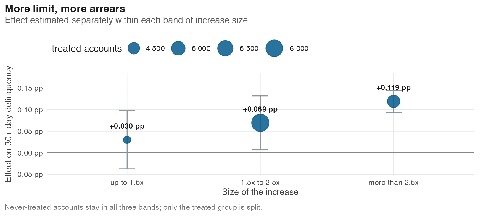
+0.030 pp for a small increase, +0.119 pp for a large one — about 4.0 times as much. A monotone dose response is another thing ordinary customer selection does not produce.
One question left: what exactly is this number?
Where this chapter’s code lives
Everything above runs from 09-why-believe.qmd. Shared setup R/_common.R. The panel itself is built by R/01-build.R.